Excel Formulas

Cells

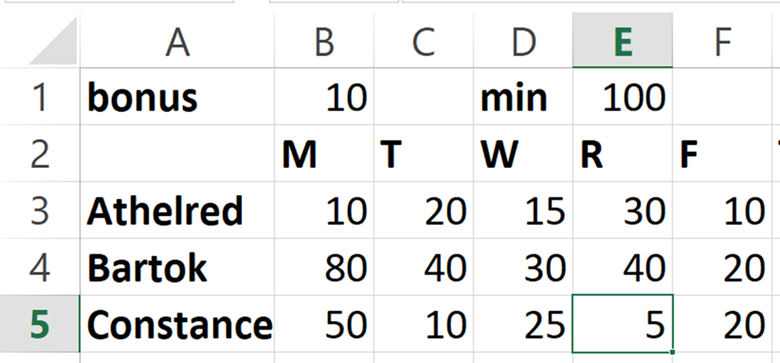
In Excel, each cell can hold a value, and the cells are organized into columns and rows. Columns are named with letters and rows with numbers. Each cell is named for its column and row, for instance the selected cell with 5 in it is cell E5

Formulas

A formula tells Excel to perform operations, such as mathematical calculation. If we put a formula in a cell, Excel will display the result of doing the operations, instead of the formula.

Formulas start with a single =. If we put the formula =10 + 5 in a cell, it will display 15. Arithmetic operators are as follows:

· Add +

· Subtract –

· Multiply *

· Divide /

If you want to see the formulas instead of their results, there is a Show Formulas button under the Formulas tab. You can also use the shortcut CTRL+~. Note that this doesn’t change what is actually in the spreadsheet, you can turn this on and off as convenient.

Cell References

Formulas are more useful if they get values from other cells, for this we use cell references, that is, use the name of another cell. So if we write =A1+B2 in a cell, we are saying to get whatever value is in A1 and whatever value is in B2, and add them together, and display the result.

If we use a reference to a cell in a formula, every time the cell is updated, the formula result will be recalculated.

Whenever possible, use a reference to another cell instead of a literal value. That way if you are using it in more than one formula in your spreadsheet, you only need to change that one cell and everything will be updated, instead of having to hunt through all your formulas to find everything you need to change.

Functions

Excel has many built-in tools called functions that you can use in your formulas. A function’s name is followed by parentheses, into which you put one or more values or cell references you want the function to operate on, its arguments[1]. If there is more than one argument, put commas between them.

For instance, the SUM function adds up its arguments, so =SUM(A1, A2, A3, A4) means, “get the values from A1, A2, A3, and A4, add them up, and display the result.” This does exactly the same thing as =A1+A2+A3+A4

If you want a function to apply to a range of cells that are next to each other, you can use a colon between the first and last reference. So =SUM(A1:A4) does exactly the same thing as =SUM(A1, A2, A3, A4) . You could also combine colons and commas, e.g. =SUM(A1:E1, A5:A25, Z1, Z25) . But commas and colons don’t do anything by themselves; =(A1:A4) is just an error

Some other useful functions that work similarly to SUM are AVERAGE, MAX, and MIN.

Note that =SUM(A1) doesn’t make sense[2]. The sum of a single number is itself, no need for SUM! Similarly =SUM(A1+A2+A3+A4) doesn’t make sense. The addition inside the parentheses happens first, and then again SUM is just trying to add up a single number. Same goes for any operations that would result in a single number inside the parentheses, e.g. =SUM(A1*A2-A3/A4).

Absolute and Relative References

Suppose I have the following data, representing commissions made by each of three employees: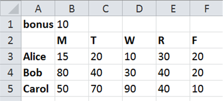

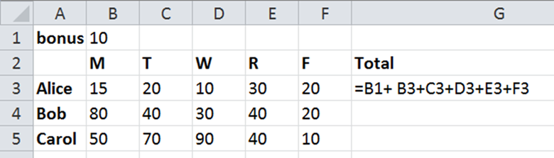
I would like to add the commissions up to see what their totals are, but I also want to include the bonus in cell B1. So I will write my first formula to find the total for Alice.

Copying Formulas

When you copy formulas in Excel from one cell to another. Excel changes the formula automatically! (Note that in Excel there is a big difference between selecting a cell then copying, and selecting the text inside a cell then copying. Here I am always referring to copying a cell, not copying some text from inside the cell.)

Excel tries to update the formula based on where you copy – if you copy to another row, it will update the row number; if you copy to a different column, it will update the column letter. It does this based on the distance and direction, so if you copy to a cell whose row number is two higher, it will add 2 to all the row numbers, if you copy to a cell whose column is two lower, it will change the letter down by 2..

So if we copy our formula to the next two cells, we get:

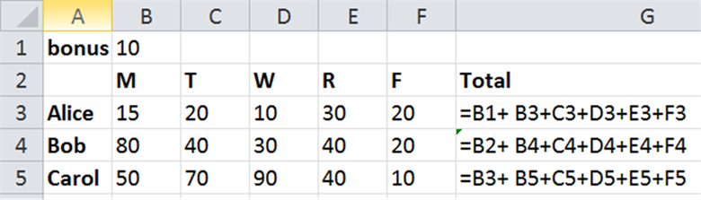
For the most part, the way Excel changes formulas is exactly what we want. But not always. Notice that while Bob and Carol’s commissions are getting added in correctly, neither of them is getting the correct bonus. We need a way to tell Excel not to change that part!

Absolute References

The references we have used so far, which Excel changes relative to where we paste formulas, are called relative references. If we want to tell Excel not to change a reference, we need absolute references.

To make a cell reference absolute, put $ in front of the parts you do not want to change. Most of the time, that means both the row and the column[3]. So A1 is a relative reference and will change on copy, $A$1 is an absolute reference and will not. So let’s change our formula to make B1 an absolute reference ($B$1) so Excel won’t change it, and then copy down again.

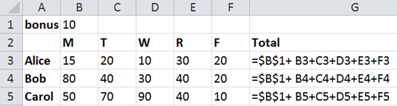
This time, Excel has left $B$1 alone, and just changed the other references.

Using IF

The built-in function IF allows us the control the value in a cell based on a yes/no question about another cell. For instance we can add a bonus only if a value is high enough.

In general, to use an IF we would say, in some cell: =if(condition, true_result, false_result)

In this formula, the condition must be something that is either true or false, using <, > <= >=, or =.

Note that we need double quotes if we are checking for text, but not for numbers

Next comes the true_result, that is, what we want the result of the formula to be if the condition was true. Finally, the false_result, what we want the result of the formula to be if the condition was false.

So if we said

• =IF(A1 > 10, “BIG”, “small”

• if the value from A1 is over 10, we’d see “BIG” and otherwise “small”

• =IF(B4 + B5 <= C10, C10, B4+B5)

• if the result of adding B4 and B5 is less than or equal to the value from C10, we’d see the value from C10, but otherwise we’d see B4+B5

• =IF(T21=60, 60, 0)

• if the value in T21 is exactly 60, we’d see 60, otherwise 0

• =IF(B17=“Dog”, “PUPPY!”, “KITTY”)

• if the value in B17 is the word Dog, we’d see “PUPPY!”, otherwise “KITTY”

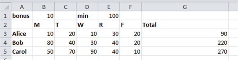
Suppose again we had the amounts made by different employees, a bonus to add, and a minimum amount we wanted them to make. Then in order to see either “Good” if they made that minimum amount, and “Poor” otherwise, we might put:

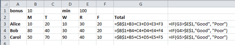
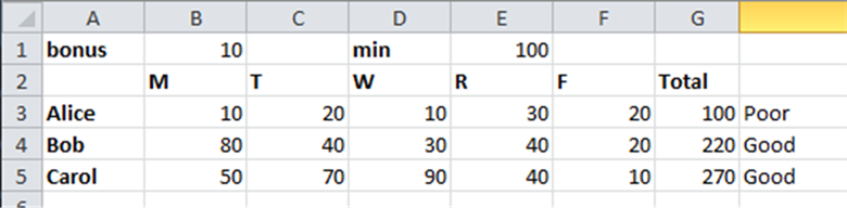
To say that if it is true that the sum (in column G) for each person is over the minimum value in E1 (note how, again, we used absolute reference) we want to see “Good” and otherwise “Poor” so we get:

Now suppose that we only want to give them the bonus if they made the minimum amount. We can include the IF function inside a formula.

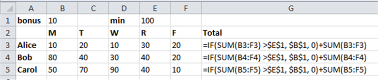
This time, instead of finding the sum with the bonus in G and then using IF on that, we are taking the sum without the bonus, and using IF to choose a value to add on. That value is the bonus from B1 if the initial sum was over the minimum, and 0 otherwise. So we get

---

[1] Different functions may accept or require different numbers of arguments, and the order of these may affect what it does.

[2] Excel will let you do this... but I will take off points using SUM without knowing how it works.

[3] $A1 tells Excel to leave the column alone but it is still okay to change the row and A$1 means it is still okay to change the column. Technically, you only need one $ if you are only changing rows or only changing columns, but it is easier to remember to just put $ on both parts