- =A1
- =A1 * 0.5
- =A1 + B2 * B3 / C4
- =(A1 + B2) * (B3 / C4)
- right: =SUM(A1, A2, A3, A4)
- right: =SUM(A1:A4)
- right: =A1 + A2 + A3 + A4
- wrong: =(A1,A2,A3,A4)
- wrong: =(A1:A4)
- stupid: =SUM(A1 + A2 + A2 + A4)
- also stupid: =SUM(B1 * B2)
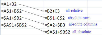
- also stupid: = SUM(B1)
Turn in your finished Excel spreadsheet attached to your Blackboard submission.
We will create a spreadsheet for estimating grades in a course.
Throughout this assignment, write your formulas so that we could go in and change the student's grade for any part or the weightings for any part and see the overall grade change automatically (that is, formulas should always use references to cells, not literal values!). Throughout this assignment, make sure everything is clearly labeled -- indicate with words what each number represents. You cannot put words in the same cell as a number you need to do calculations on.
Part A
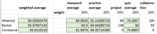
In a certain course, student grades depend on classwork (30%) practice (20%) a project (20%) quizzes (20%) and collaboration (10%)
Set up an Excel spreadsheet with names of three students down the first column, and titles for columns across the top, as well as percentages in the next row down (as shown below).
In the picture below, the boxed cells are the results of formulas you will need to write, while the non-boxed cells can just be made up numbers. You can fill in the made up numbers now (using mine or others that amuse you)
Part B
Further to the right from this part of the spreadsheet, on the first student's row in the spreadsheet, we will add more grades, so we can compute the rest of the students' averages instead of using made-up numbers:
☑ For the first student, give them three classwork grades, three practice grades, and three quiz grades, each labeled -- you can have just one "classwork" entry and then use numbers to label the rest. (When making up grades, they don't have to all be different.)
☑ Add formulas in the first student's row to calculate (not weighted) averages for averages of those grades.
☑ Do the same for the other two students, copying the formulas down (do you need absolute references for this?).
Part C
☑ Next we will calculate the overall grade for the first student, based on the weightings for this class. To compute a weighted average, we multiply the value for each part times the weight for that part, then add them all up.
So, if a student had a 90 average on classwork, a 100 average on practices, an 88 on the project, 79 average on quizzes, and 50 on collaboration, their overall grade would be:
90 *.30 +
100 * .20 +
88 *.20 +
79 *.20 +
50 * .10
☑ Write a formula to do this for the first student, using their grades (based on the cells in their row), and the weights (based on the weight row).
☑ We want to copy that formula for the other students. Adjust your formula, using absolute and relative references appropriately, so that it will copy correctly to the other rows, so the copies will use each of the other students' grades, but still use the same weights from the original row. Then do copy it to the other other students' rows.
☑ In the column after the names use an if formula to choose whether to show "ok" or "F" depending on if the student is failing (weighted average under 60%).
[EC+10] Add seperate entries for both job and problem projects. Enter a formula for the first student's project grade to be the average for the job project grade + 50% * the problem project grade. This is a "normal" add-up-and-divide average, not a weighted average. Copy the formula down for the other students.